Demo on Differential Equations, Math 141, Fall 2012
Contents
Direction Fields
Say we want to study an equation like

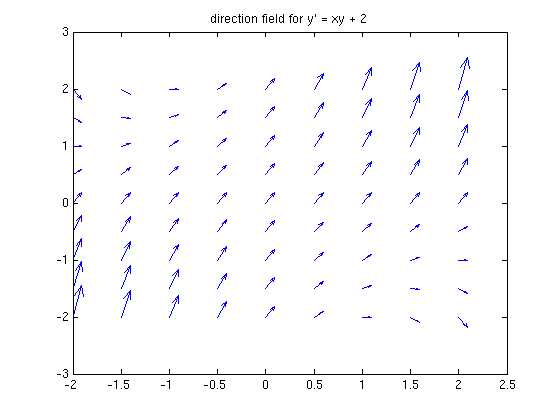
We can start by drawing a "direction field", showing the slopes  at various points.
[xx, yy] = meshgrid(-2:.5:2, -2:.5:2);
quiver(xx, yy, ones(size(xx)), xx.*yy + 2)
title 'direction field for y'' = xy + 2'
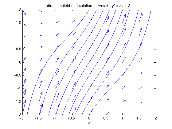
From the picture, we can visualize what the solutions look like. We can also solve for them analytically:
syms x c
sol = dsolve('Dy = x*y + 2', 'y(0) = c', 'x')
sol =

c*exp(x^2/2) + 2^(1/2)*pi^(1/2)*exp(x^2/2)*erf((2^(1/2)*x)/2)
Solution Curves
The answer is in terms of a constant of integration c. Let's plot the solutions for different values of c on the same axes.
hold on
for j = -2:.5:2
    ezplot(subs(sol, c, j), [-2, 2]), axis([-2, 2, -2 2])
end
hold off
title 'direction field and solution curves for y'' = xy + 2'
Nonlinear Equations
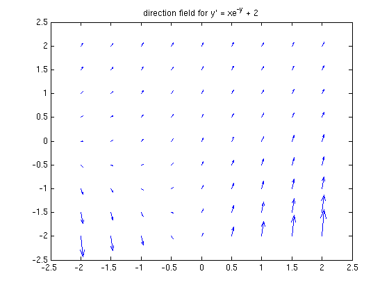
The equation above is linear, which implies that there is a closed-form solution. When an equation is non-linear, as in the following example

it may or may not be possible to solve explicitly, though one can always solve numerically given an initial condition. Here is the "direction field", showing the slopes at various points.
quiver(xx, yy, ones(size(xx)), xx.*exp(-yy) + 2)
title 'direction field for y'' = xe^{-y} + 2'
sol1 = dsolve('Dy = x*exp(-y) + 2', 'y(0) = c', 'x')
sol1 =

- log(-1/(2*x - 4*exp(2*x)*(exp(c) + 1/4) + 1)) - 2*log(2)
Let's superimpose some solution curves.
hold on
for j = -2:.5:2
    ezplot(subs(sol1, c, j), [-2, 2]), axis([-2, 2, -2 2])
end
hold off
title 'direction field and solution curves for y'' = xe^{-y} + 2'
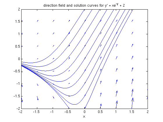
In this case the solution curves at the top of the picture all look like straight lines. This makes sense, since for y large,  is almost 0, and so the equation looks like
  , which has solution curves of the form
  .
.