Geometry of Curves
copyright  2011 by Jonathan Rosenberg
based on an earlier M-book, copyright 2000-2003 by Paul Green and Jonathan Rosenberg. In this published M-file, we will use MATLAB to perform computations and obtain plots involving parametrized curves in two and three dimensions.
Contents
Plane Curves
We begin by considering the cycloid, which you have already seen in the text of Ellis and Gulick. It is parametrized by (t - sin(t), 1 - cos(t)). Let us enter this information into MATLAB. We enter the cycloid as a three dimensional curve in order to be able to use the cross-product later on.
syms t real
cycloid=[t-sin(t),1-cos(t),0]
cycloid =

[ t - sin(t), 1 - cos(t), 0]
Let us compute the velocity and acceleration (i.e., the first two derivatives), the speed and the curvature for the cycloid. We will differentiate symbolically with respect to t; however, we do not need to specify t as an argument to diff because MATLAB will automatically differentiate with respect to the variable nearest to x alphabetically, and there is only one variable in this case. First we define a function veclength for computing Euclidean lengths of vectors. We don't want to call it length or norm since those names are already reserved by MATLAB for other purposes.
veclength = @(v) sqrt(dot(v,v))
veclength =

    @(v)sqrt(dot(v,v))
First we compute the velocity, acceleration, and speed:
cycvel = diff(cycloid)
cycacc = diff(cycvel)
cycspeed = simplify(veclength(cycvel))
cycvel =

[ 1 - cos(t), sin(t), 0]


cycacc =

[ sin(t), cos(t), 0]


cycspeed =

2^(1/2)*(1 - cos(t))^(1/2)
From all this we can compute the curvature:
cyccurve = veclength(cross(cycvel,cycacc))/cycspeed^3
cyccurve =

(2^(1/2)*((cos(t) - 1)^2)^(1/2))/(4*(1 - cos(t))^(3/2))
We can use the pretty command to improve the appearance and intelligibility of the formula for the curvature.
pretty(cyccurve)
   1/2              2 1/2
  2    ((cos(t) - 1) )
  -----------------------
                    3
                    -
                    2
      4 (1 - cos(t))
Note that the numerator contains a square followed by a square root, in other words an absolute value. We can get things into better form using simple:
cyccurve=simple(cyccurve)
cyccurve =

2^(1/2)/(4*(1 - cos(t))^(1/2))
The numerator here contains (cos(t) - 1)^2)^(1/2), which since cos(t) <= 1 is just 1 - cos(t). This cancels part of the denominator so we can really write:
cyccurve=(1/2)/(2-2*cos(t))^(1/2)
cyccurve =

1/(2*(2 - 2*cos(t))^(1/2))
Problem 1:
Find symbolic expressions for the velocity, speed, acceleration and curvature for the hypocycloid parametrized by:
hypocyc=[2*cos(t)+cos(2*t),2*sin(t)-sin(2*t),0]
hypocyc =

[ cos(2*t) + 2*cos(t), 2*sin(t) - sin(2*t), 0]
We continue our study of the cycloid. Let us plot it. We use ezplot, which will plot a parametrized plane curve provided the first two arguments are the coordinate functions. The last argument gives the range of the parameter for the plot. The command axis normal changes ezplot's default scaling, which would have set the scales on the two axes to be equal.
ezplot(cycloid(1),cycloid(2),[0,4*pi]);axis normal
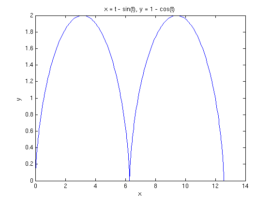
We have shown two arches of the cycloid in order to show the cusp at (2π, 0). There are two natural questions. One is the length of each arch, and the other is the behavior of the curvature at the cusp. The length of the cycloid can be computed symbolically, by integrating the speed.
cyclength=int(cycspeed,0,2*pi)
cyclength =

8
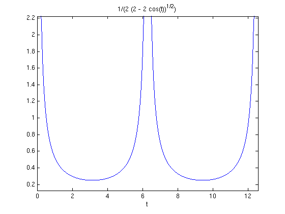
Of course, 4^(1/2) is really 2, so this is the (exact) number 8. However, MATLAB does not simplify 4^(1/2) to 2 since it doesn't know for sure that we want the positive, rather than negative, square root. Now let us look more carefully at the curvature

which clearly becomes infinite as cos(t) approaches 1. This behavior is not apparent from the plot, which makes it look as though the curve becomes straight near the cusp. However it does become apparent from a plot of the curvature as a function of t.
ezplot(cyccurve,[0,4*pi])
Let us see what we can learn by making a detailed plot near the cusp. We will use the cusp at the origin for the sake of simplicity.
ezplot(cycloid(1),cycloid(2),[-.1,.1]);axis normal

ezplot(cycloid(1),cycloid(2),[-.01,.01]);axis normal
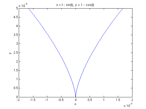
ezplot(cycloid(1),cycloid(2),[-.001,.001]);axis normal
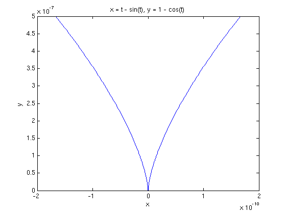
In order to interpret these plots, which appear to be quite similar, we begin by recalling that the curvature of a plane curve can be identified with

where phi is the angle between the unit tangent and any convenient reference ray. In this case we choose our reference ray to be the positive y-axis. Then for small values,
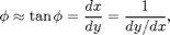
because our reference line is vertical instead of horizontal. Now , the change in across our plotting interval, appears to be the same in all three plots, as does , the length of the plotted curve. However, if we look at the scales on the axes, we observe that as the length of the plotting interval decreases by a factor of 10, the y-scale decreases by a factor of 100 and the x-scale decreases by a factor of 1000. Since the y-scale dominates, we can identify with , so that also decreases by a factor of 100. On the other hand, the ratio between the apparent angle with the positive y-axis and the actual angle scales with the ratio of the x-scale to the y-scale. This only decreases by a factor of 10. Thus as the length of the plotting interval decreases by a factor of 10, the ratio increases by a factor of 10, showing that the curvature approaches as t approaches 0.
Space Curves, Frenet Frames, and Torsion
In this section, we will plot curves in 3-dimensional space and compute their invariants. As we proceed we will provide a detailed discussion of some mathematical concepts that are not mentioned in Ellis and Gulick. In order to have a concrete example before us, we consider the twisted cubic, parametrized by:

syms t
twistcube=[t,t^2,t^3]
twistcube =

[ t, t^2, t^3]
It will be convenient to define a MATLAB function unitvec which converts a vector to a unit vector by dividing the vector by its length:
unitvec = @(v) v/veclength(v)
unitvec =

    @(v)v/veclength(v)
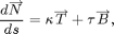
The Frenet frame of a curve at a point is a triple of vectors (T, N, B) consisting of the unit tangent vector T at that point, the unit normal N (the unit vector in the direction of the derivative of the unit tangent), and the unit binormal B = T ? N, the cross-product of the unit tangent with the unit normal. We calculate the Frenet frame for the twisted cubic:
tcvel=diff(twistcube)
tctan=simplify(unitvec(tcvel))
tcacc=diff(tcvel)
tcvel =

[ 1, 2*t, 3*t^2]


tctan =

[ 1/(9*t^4 + 4*t^2 + 1)^(1/2), (2*t)/(9*t^4 + 4*t^2 + 1)^(1/2), (3*t^2)/(9*t^4 + 4*t^2 + 1)^(1/2)]


tcacc =

[ 0, 2, 6*t]
Because the acceleration a is not parallel to the unit normal N, but the cross-product v ? a of the velocity and the acceleration is parallel to the unit binormal B, it is convenient to compute the unit binormal before the unit normal vector.
tccross=cross(tcvel,tcacc)
tcbin=simplify(unitvec(tccross))
tccross =

[ 6*t^2, -6*t, 2]


tcbin =

[ (3*t^2)/(9*t^4 + 9*t^2 + 1)^(1/2), -(3*t)/(9*t^4 + 9*t^2 + 1)^(1/2), 1/(9*t^4 + 9*t^2 + 1)^(1/2)]
Since T is perpendicular to N and B = T ? N, the three unit vectors T, N, and B are mutually perpendicular, and it follows that also N = B ? T and T = N ? B. This gives the fastest way to compute N.
tcnorm = simplify(cross(tcbin, tctan))
tcnorm =

[ -(t*(9*t^2 + 2))/((9*t^4 + 4*t^2 + 1)^(1/2)*(9*t^4 + 9*t^2 + 1)^(1/2)), -(9*t^4 - 1)/((9*t^4 + 4*t^2 + 1)^(1/2)*(9*t^4 + 9*t^2 + 1)^(1/2)), (3*t*(2*t^2 + 1))/((9*t^4 + 4*t^2 + 1)^(1/2)*(9*t^4 + 9*t^2 + 1)^(1/2))]
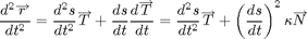
We recall that the curvature, while defined as the magnitude of the derivative of the unit tangent with respect to arclength, is most conveniently computed as follows:
tccurve=simplify(veclength(tccross)/veclength(tcvel)^3)
tccurve =

(2*(9*t^4 + 9*t^2 + 1)^(1/2))/(9*t^4 + 4*t^2 + 1)^(3/2)
Problem 2:
Consider the trefoil parametrized by
trefoil=[(2+cos(3*t))*cos(2*t),(2+cos(3*t))*sin(2*t),cos(3*t)]
trefoil =

[ cos(2*t)*(cos(3*t) + 2), sin(2*t)*(cos(3*t) + 2), cos(3*t)]
- (a) Plot the trefoil for t between 0 and 2pi.
- (b) Compute the curvature of the trefoil.
- (c) Compute the Frenet frame of the trefoil.
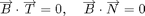
We could also have defined the curvature as the normal component of the derivative of the unit tangent with respect to arclength. The two definitions are synonymous because the derivative of the unit tangent, either with respect to the parameter t or with respect to arclength s, is parallel to the unit normal. Symbolically, what we have so far, if Greek kappa denotes the curvature, is


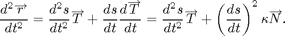
From this it follows, since T ? T = 0, that
which explains the formula for the curvature.
We are now interested in the derivative of the unit normal with respect to arclength. By differentiating the equation

with respect to s, we obtain
from which it follows that

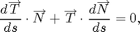
Since N is a unit vector, we know that

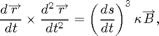
is perpendicular to N. The torsion is defined to be

Note that since the direction of B is determined independently of

the torsion, unlike the curvature, is signed. Notice also that for a plane curve, the binormal is identically perpendicular to the plane in which the curve lies, and thus the torsion is 0. Thus we have the Frenet-Serret formulae:


The last of these is easily obtained by differentiating the equations
with respect to s. Now we want to obtain a more computable formula for the torsion. We begin by differentiating the equation
which we established earlier. The product and chain rules will generate many terms, but the only one that is not perpendicular to B is the one that comes from differentiating N. Thus we have

Now comparing with the formula

we obtain
which is a convenient formula for the torsion. In the case of the twisted cubic, it gives
tcthird=diff(tcacc)
tctors=simplify(dot(tccross,tcthird)/dot(tccross,tccross))
tcthird =

[ 0, 0, 6]


tctors =

3/(9*t^4 + 9*t^2 + 1)
Problem 3:
Compute the torsion of the trefoil.
To begin to see the geometrical significance of the torsion, we use the M-file curveframeplot.m,available at http://www.math.umd.edu/users/jmr/241/mfiles/curveframeplot.m. This plots the curve in blue together with normal vectors in red and binormal vectors in green. The tangent vectors are not plotted since the tangent direction is clear from the curve. The last two arguments determine the number of frames plotted and the length of the normal and binormal vectors.
type curveframeplot
% This is an M-file intended to plot a space curve together with
% several instances of the Frenet Frame, represented by the
% normal in red and the unit binormal in green. The
% parameter num determines the number of frames plotted; the
% parameter len determines the length of the frame vectors.

function  z = curveframeplot(curve, parameter, start, fin, num, len)

newcurve=subs(curve, parameter, 't');
t= start:.01*(fin-start):fin;
x = eval(vectorize(newcurve(1)));
y = eval(vectorize(newcurve(2)));
w = eval(vectorize(newcurve(3)));
plot3(x,y,w)
hold on

unitvec = @(u) u/sqrt(u*transpose(u));
curvevel=diff(curve);
curvetan=unitvec(curvevel);
curvenorm=unitvec(diff(curvetan));
curvebin=cross(curvetan,curvenorm);

t1=start:(fin-start)/num:fin;
newcurve1=subs(curve,parameter,'t1');
norm1=subs(curvenorm,parameter,'t1');
bin1=subs(curvebin,parameter,'t1');
x1 = eval(vectorize(newcurve1(1)));
y1 = eval(vectorize(newcurve1(2)));
w1 =eval(vectorize(newcurve1(3)));
xnorm = eval(vectorize(newcurve1(1)+len*norm1(1)));
ynorm = eval(vectorize(newcurve1(2)+len*norm1(2)));
wnorm=eval(vectorize(newcurve1(3)+len*norm1(3)));
xbin = eval(vectorize(newcurve1(1)+len*bin1(1)));
ybin = eval(vectorize(newcurve1(2)+len*bin1(2)));
wbin =eval(vectorize(newcurve1(3)+len*bin1(3)));

for n=1:length(t1)
   plot3([x1(n),xnorm(n)],[y1(n),ynorm(n)],[w1(n),wnorm(n)],'red')
   plot3([x1(n),xbin(n)],[y1(n),ybin(n)],[w1(n),wbin(n)],'green')
end
hold off
curveframeplot(twistcube,'t',-1,1,10,.2)
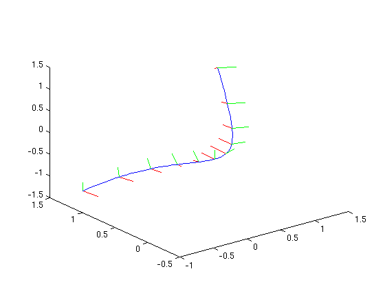
Notice how the Frenet frames twist around the curve as the parameter changes. To make this even clearer, we define and plot a tube around the curve. We will need a second parameter since the tube is a surface.
syms s
tctube=twistcube+ .2*cos(s)*tcnorm+.2*sin(s)*tcbin ;
pretty(tctube)
  +-                                                                                                                                                                                                                                -+
  |              2                                         2                                                                         4                                                                            2                  |
  |           3 t  sin(s)                     t cos(s) (9 t  + 2)               2         3 t sin(s)                      cos(s) (9 t  - 1)                       sin(s)            3              3 t cos(s) (2 t  + 1)             |
  |  t + ---------------------- - -------------------------------------------, t  - ---------------------- - -------------------------------------------, ---------------------- + t  + -------------------------------------------  |
  |            4      2     1/2         4      2     1/2     4      2     1/2             4      2     1/2         4      2     1/2     4      2     1/2        4      2     1/2              4      2     1/2     4      2     1/2  |
  |      5 (9 t  + 9 t  + 1)      5 (9 t  + 4 t  + 1)    (9 t  + 9 t  + 1)          5 (9 t  + 9 t  + 1)      5 (9 t  + 4 t  + 1)    (9 t  + 9 t  + 1)     5 (9 t  + 9 t  + 1)           5 (9 t  + 4 t  + 1)    (9 t  + 9 t  + 1)     |
  +-                                                                                                                                                                                                                                -+
In this case, the input is more illuminating than the output. For fixed t, s parametrizes a circle around the tube. For fixed s, t parametrizes a curve running along the tube and, in the presence of torsion, twisting around it. We will plot the tube using ezmesh. The first three arguments are the components of tctube; the last argument gives the limits for s and t in the form [smin, smax, tmin, tmax]:
ezmesh(tctube(1),tctube(2),tctube(3),[0,2*pi,-1,1])
title('Tube around a twisted cubic')
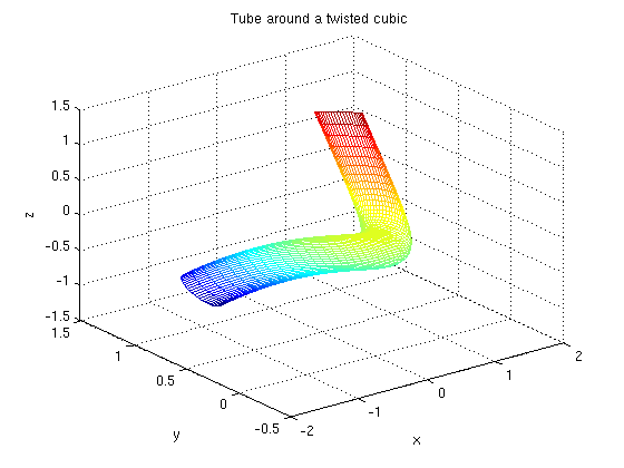
The torsion is illustrated by the way in which the longitudinal mesh lines, corresponding to constant values of s, twist around the tube.
Problem 4:
- (a) Use curveframeplot to plot the trefoil with its Frenet frame.
- (b) Use ezsurf to show the twisting of the Frenet frame of the trefoil around the curve.
Additional Problems:
- 1) Observe that any curve given in polar coordinates by a function f can be parametrized as (f(t)cos(t), f(t)sin(t)). Use this observation to analyze each of the following curves. Plot each curve, compute its length, plot the curvature as a function of t, determine the curvature bounds, and identify any cusps or self-intersections:
- The cardioid

- The lemniscate

- The limacon

- 2) Observe that the graph of a function f can be parametrized as (t, f(t)). Use this observation to analyze the graph of each of the following functions. Determine the curvature bounds if they exist, compute the length of each graph between x = 0 and x = 1, and identify any cusps:
- x^2
- x^3
- x^4
- x^(3/2)
- e^x
- 3) Consider the family of helices parametrized by (R cos(t), R sin(t), A t).
- (a) Compute the torsion and curvature as functions of R and A.
- (b) For R = A = 1, plot the helix, showing the Frenet frame at several points along the curve.
- (c) Plot the tube of radius .2 around the helix showing the twisting of the Frenet frame around the helix.
- 4) Consider the curve parametrized by
- (a) Compute the torsion and the binormal.
- (b) What do you deduce about the curve from the result of part a)?
- (c) Provide a graphical demonstration of your conclusion in part b).