Graphical-Numerical Optimization Methods and Lagrange Multipliers
copyright © 2009 by Jonathan Rosenberg based on an earlier M-book copyright © 2000 by Paul Green and Jonathan Rosenberg
Contents
Constrained Extremal Problems in Two Variables
In this published M-file, we will examine the problem of finding the extreme values of a function on a bounded region. We will start by finding the extreme values of the function
on the region
Extreme values can occur either at critical points of f interior to the region, or along the boundary. What we must do, therefore, is evaluate f at those critical points that satisfy the inequality defining the region, and compare those values to the maximum and minimum along the boundary. We will find the latter by using the method of Lagrange multipliers. We begin by defining the functions f and g in MATLAB.
syms x y z
f=4-x^2-y^2+x^4+y^4
g=exp(x^2)+2*exp(y^2)
f =

x^4 - x^2 + y^4 - y^2 + 4


g =

exp(x^2) + 2*exp(y^2)
Next, we find the critical points of f. For reasons that will become apparent later, we include the derivative of f with respect to z, even though it is identically 0 since f does not depend on z.
gradf=jacobian(f,[x,y,z])
[xfcrit,yfcrit]=solve(gradf(1),gradf(2));
[xfcrit,yfcrit]
gradf =

[ 4*x^3 - 2*x, 4*y^3 - 2*y, 0]


ans =

[          0,          0]
[          0,  2^(1/2)/2]
[  2^(1/2)/2,          0]
[ -2^(1/2)/2,          0]
[          0, -2^(1/2)/2]
[  2^(1/2)/2,  2^(1/2)/2]
[ -2^(1/2)/2,  2^(1/2)/2]
[  2^(1/2)/2, -2^(1/2)/2]
[ -2^(1/2)/2, -2^(1/2)/2]
Next, we evaluate g at the critical points to determine which of them are in the region.
gfun=@(x,y) eval(vectorize(g))
double(gfun(xfcrit,yfcrit))
gfun =

    @(x,y)eval(vectorize(g))


ans =

    3.0000
    4.2974
    3.6487
    3.6487
    4.2974
    4.9462
    4.9462
    4.9462
    4.9462
We see that only the first three critical points are in the region. Consequently we are only interested in the values of f at those points.
ffun=@(x,y) eval(vectorize(f))
ffun(xfcrit(1:3),yfcrit(1:3))
ffun =

    @(x,y)eval(vectorize(f))


ans =

    4
 15/4
 15/4
We must now address the problem of finding the extreme values of f on the boundary curve. The theory of Lagrange multipliers tells us that the extreme values will be found at points where the gradients of f and g are parallel. This will be the case precisely when the cross-product of the gradients of f and g is zero. It is for this reason that we have defined the gradient of f, and will define the gradient of g, to be formally three-dimensional. We observe that since the gradients of f and g lie in the plane (spanned by i and j), only the third component of the cross-product,
will ever be different from zero. This gives us a system of two equations, the solutions of which will give all possible locations for the extreme values of |f |on the boundary.
gradg=jacobian(g,[x,y,z])
gradcross=cross(gradf,gradg);
lagr=gradcross(3)
gradg =

[ 2*x*exp(x^2), 4*y*exp(y^2), 0]


lagr =

2*x*exp(x^2)*(2*y - 4*y^3) - 4*y*exp(y^2)*(2*x - 4*x^3)
[xboundcrit,yboundcrit]=solve(g-4,lagr)
xboundcrit =

0.60004900866399495492018052548414


yboundcrit =

0.4994292157542333618021166445329
MATLAB was unable to find all constrained critical points. We shall have to resort to graphical-numerical methods. We begin by plotting the loci of the two equations we are trying to solve.
[xx, yy] = meshgrid(-2:.05:2,-2:.05:2);
gfun = inline(vectorize(g));
lagfun = @(x,y) eval(vectorize(lagr));
contour(xx, yy, gfun(xx, yy), [4,4], 'r'); hold on;
contour(xx, yy, lagfun(xx, yy), [0,0], 'b'); hold off;
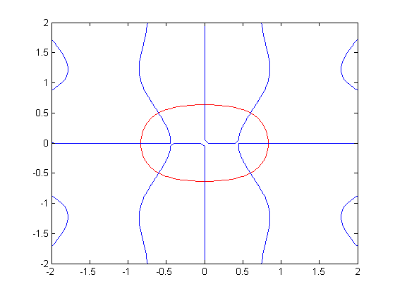
We see now that there are eight critical points. Four of them are on the axes, and can be easily be found analytically. The other four will require the use of the root finder newton2d from the last lesson. Let us deal with the first four. We simply have to set x or y to zero and solve the equation g = 4 for the other variable. This gives
xaxiscrits=solve(subs(g-4,y,0));
[xaxiscrits,[0;0]]
ans =

[ -log(2)^(1/2), 0]
[  log(2)^(1/2), 0]
yaxiscrits=solve(subs(g-4,x,0));
[[0;0],yaxiscrits]
ans =

[ 0, -log(3/2)^(1/2)]
[ 0,  log(3/2)^(1/2)]
The numerical values of these critical points are:
double([xaxiscrits,[0;0]])
double([[0;0],yaxiscrits])
ans =

   -0.8326         0
    0.8326         0


ans =

         0   -0.6368
         0    0.6368
and the corresponding f-values are:
double(ffun(xaxiscrits,[0;0]))
double(ffun([0;0],yaxiscrits))
ans =

    3.7873
    3.7873


ans =

    3.7589
    3.7589
The remaining four constrained critical points seem to be near

[xb1,yb1]=newton2d(g-4,lagr,.5,.5); [xb1,yb1]
[xb2,yb2]=newton2d(g-4,lagr,-.5,.5); [xb2,yb2]
[xb3,yb3]=newton2d(g-4,lagr,-.5,-.5); [xb3,yb3]
[xb4,yb4]=newton2d(g-4,lagr,.5,-.5) ; [xb4,yb4]
ffun([xb1,xb2,xb3,xb4],[yb1,yb2,yb3,yb4])
ans =

    0.6000    0.4994


ans =

   -0.6000    0.4994


ans =

   -0.6000   -0.4994


ans =

    0.6000   -0.4994


ans =

    3.5824    3.5824    3.5824    3.5824
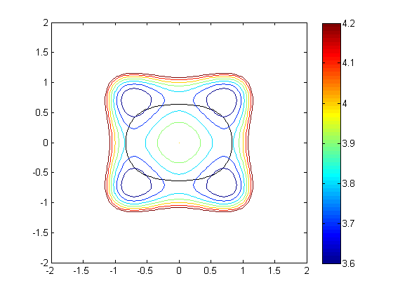
We now see that the maximum value of f in the region of interest is 4, at the interior critical point (0,0), and the minimum value is 3.5824, taken at the four points we just found. We can check this graphically by superimposing a contour plot of f on a picture of the bounding curve. Note that we select only those contours of f with values close the ones we want, in order to get the best possible picture, and have added the colorbar command to add a legend indicating what colors correspond to what f-values.
contour(xx, yy, gfun(xx, yy), [4,4], 'k'); hold on;
contour(xx, yy, ffun(xx, yy), [3:.1:4.2]); hold off;
colorbar
Problem:
Find the minimum and maximum values of the function

on the region defined by

A Physical Application
Here's an example from quantum mechanics that illustrates how the Lagrange multiplier method can be used. Consider a particle of mass m free to move along the x-axis, sitting in a "potential well" given by a potential energy function V(x) that tends to +infinity as x tends to plus or minus infinity. Then the "ground state" of the particle is given by a "wave function" φ(x), where

gives the probability density of finding the function near x. Since the total probability of finding the function somewhere is 1, we have the constraint that the integral of φ(x)^2 must be 1. A basic principle of physics states that phi(x) will be the function minimizing the energy E(φ), which is given by
![$$ E(\phi) = \int_{-\infty}^{\infty} \left[\frac{h^2}{2m}\phi'(x)^2 + V(x)\phi(x)^2\right]\,dx,$$](lagrange_eq43137.png)
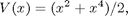
where h is Planck's constant. Usually it's not possible to find the function exactly, but a convenient way of approximating it is to guess a form for phi(x) involving some parameters, and then adjust the parameters to minimize E(φ) subject to the constraint that the integral of phi(x)^2 is = 1. For simplicity let's take h=m=1. Say for example that V(x) = x^4/2 (the "anharmonic" oscillator). Let's choose a reasonable form for a function phi(x) that dies rapidly at infinity. By symmetry, phi(x) has to be an even function of x, so let's try:
syms a b c
phi=a*exp(-x^2)*(1+b*x^2+c*x^4)
g=simple(int(phi^2, -inf, inf))
phi =

(a*(c*x^4 + b*x^2 + 1))/exp(x^2)


g =

(2^(1/2)*pi^(1/2)*a^2*(48*b^2 + 120*b*c + 128*b + 105*c^2 + 96*c + 256))/512
So our constraint is g = 1. Now let's compute the energy function. (For convenience we're leaving out the factor of 1/2 in both terms inside the integral.)
phiprime=simple(diff(phi))
energy=simple(int(phiprime^2+x^4*phi^2,-inf,inf))
phiprime =

-(2*a*x*(b*x^2 - b - 2*c*x^2 + c*x^4 + 1))/exp(x^2)


energy =

(2^(1/2)*pi^(1/2)*a^2*(3472*b^2 + 10248*b*c - 128*b + 13995*c^2 - 1248*c + 4864))/8192
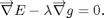
Now we solve the Lagrange multiplier equations. This time we have a function E(a,b,c) that we need to minimize subject to a constraint g(a,b,c) = 1, so the equations are
syms lam
eg=jacobian(energy,[a,b,c]);
gg=jacobian(g,[a,b,c]);
lagr=eg-lam*gg;
[asol,bsol,csol,lsol]=solve(g-1,lagr(1),lagr(2),lagr(3),a,b,c,lam);
double([asol,bsol,csol,lsol])
ans =

  Columns 1 through 3

   0.5971            -7.5249             4.8791 - 0.0000i
  -0.5971            -7.5249             4.8791 - 0.0000i
   0.7902             0.5222            -0.0577 + 0.0000i
  -0.7902             0.5222            -0.0577 + 0.0000i
   0.7177            -3.1700            -0.2087 + 0.0000i
  -0.7177            -3.1700            -0.2087 + 0.0000i

  Column 4

  16.7155
  16.7155
   1.0611
   1.0611
   7.5359
   7.5359
Clearly there's some small imaginary round-off error here. We can get rid of it by taking the real parts:
real(double([asol,bsol,csol,lsol]))
ans =

    0.5971   -7.5249    4.8791   16.7155
   -0.5971   -7.5249    4.8791   16.7155
    0.7902    0.5222   -0.0577    1.0611
   -0.7902    0.5222   -0.0577    1.0611
    0.7177   -3.1700   -0.2087    7.5359
   -0.7177   -3.1700   -0.2087    7.5359
Now we need to look for the minimum value of the energy:
efun=@(a,b,c) eval(vectorize(energy));
real(double(efun(asol,bsol,csol)))
ans =

   16.7155
   16.7155
    1.0611
    1.0611
    7.5359
    7.5359
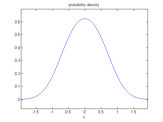
The minimum energy for this choice of the form of phi(x) is thus 1.0611. We can plot the probability density:
bestphi=subs(phi,[a,b,c],double([asol(3),bsol(3),csol(3)]));
ezplot(bestphi^2); title('probability density')
Additional Problems
- 1. Find the minimum value of the function

subject to the constraint

You will find many interior critical points and many solutions to the Lagrange multiplier equations.
- 2. Find and plot the function φ(x) (of the same form as in the example above) minimizing the energy for the potential
with the same constraint that the integral of phi(x)^2 = 1, and compare the result with the example above. Again take h = m = 1.